This tutorial walks through the examples/magnitude_spectrum.c program, which generates a multi-tone signal, windows it, computes the magnitude spectrum with MD_magnitude_spectrum(), and visualises the result.

What is a magnitude spectrum?

Every real-valued signal can be decomposed into a sum of sinusoids at different frequencies. The magnitude spectrum tells you the amplitude of each sinusoidal component.

The tool for this decomposition is the Discrete Fourier Transform (DFT). Given \(N\) samples \(x[n]\), the DFT produces \(N\) complex coefficients:

\[ X(k) = \sum_{n=0}^{N-1} x[n] \, e^{-j\,2\pi\,k\,n/N}, \qquad k = 0, 1, \ldots, N-1 \]

The magnitude spectrum is simply the absolute value of these coefficients: \(|X(k)|\). Each bin \(k\) corresponds to frequency \(f_k = k \cdot f_s / N\), where \(f_s\) is the sample rate.

For a real signal, the spectrum is symmetric around \(N/2\), so only the first \(N/2 + 1\) bins (the "one-sided" spectrum) carry unique information.

Step 1: Generate a test signal

We create a signal with three known sinusoidal components (440 Hz, 1000 Hz, and 2500 Hz) at different amplitudes, plus a small DC offset. This lets us verify that the spectrum shows peaks at exactly those frequencies.

    double *tone = malloc(N * sizeof(double));
    for (unsigned i = 0; i < N; i++) signal[i] = dc;
 
    MD_sine_wave(tone, N, amp1, freq1, sample_rate);
    for (unsigned i = 0; i < N; i++) signal[i] += tone[i];
 
    MD_sine_wave(tone, N, amp2, freq2, sample_rate);
    for (unsigned i = 0; i < N; i++) signal[i] += tone[i];
 
    MD_sine_wave(tone, N, amp3, freq3, sample_rate);
    for (unsigned i = 0; i < N; i++) signal[i] += tone[i];
 
    free(tone);

Step 2: Apply a window function

Before computing the FFT, we multiply the signal by a Hanning window. Why?

The DFT assumes the input is one period of a periodic signal. In reality, our signal chunk rarely starts and ends at a perfect zero crossing. This mismatch creates an artificial discontinuity at the boundaries, which causes energy to "leak" from the true frequency into neighbouring bins – an effect called spectral leakage.

A window function tapers the signal smoothly to zero at both edges, eliminating the discontinuity:

\[ w[n] = 0.5 \left(1 - \cos\!\left(\frac{2\pi\,n}{N-1}\right)\right) \]

    MD_Gen_Hann_Win(window, N);
    for (unsigned i = 0; i < N; i++) {
        windowed[i] = signal[i] * window[i];
    }

The trade-off: windowing widens the main lobe of each peak slightly (reducing frequency resolution) but dramatically suppresses the side lobes (improving dynamic range).

Step 3: Compute the magnitude spectrum

With the windowed signal ready, a single call to MD_magnitude_spectrum() computes \(|X(k)|\) for bins \(k = 0, 1, \ldots, N/2\):

MD_magnitude_spectrum(windowed, N, mag);

MD_magnitude_spectrum

void MD_magnitude_spectrum(const double *signal, unsigned N, double *mag_out)

Compute the magnitude spectrum of a real-valued signal.

Definition minidsp.c:727

Internally, miniDSP uses FFTW to compute the real-to-complex FFT, then takes the absolute value of each complex coefficient.

Step 4: Convert to a one-sided amplitude spectrum

The raw magnitudes \(|X(k)|\) are unnormalised (they scale with \(N\)). To recover the actual signal amplitudes, we:

**Divide every bin by \(N\)** to undo the DFT scaling.
Double the interior bins ( \(k = 1 \ldots N/2-1\)) because the energy from the discarded negative-frequency bins folds onto the positive side.
Leave DC and Nyquist alone – they have no mirror image.

    for (unsigned k = 0; k < num_bins; k++) {
        freqs[k] = (double)k * sample_rate / (double)N;
        mag[k] /= (double)N;
        if (k > 0 && k < N / 2) {
            mag[k] *= 2.0;
        }
    }

After this normalisation, a pure sine wave at amplitude \(A\) produces a peak of height \(A\) in the spectrum.

Results

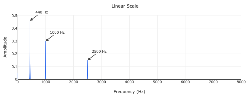
Linear scale

The linear-scale plot shows clear spikes at the three input frequencies. The 440 Hz tone (amplitude 1.0) is tallest, followed by 1000 Hz (0.6) and 2500 Hz (0.3). The tiny spike at 0 Hz is the DC offset (0.1).

Magnitude spectrum -- linear scale

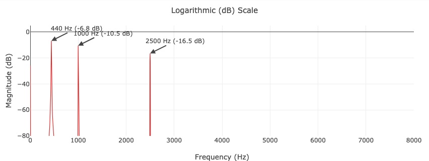
Logarithmic (dB) scale

The dB plot reveals low-level details invisible on the linear scale. The Hanning window's side lobes appear as the gradually decaying skirt around each peak. Without windowing, these lobes would be much higher and wider, obscuring nearby weak signals.

Magnitude spectrum -- dB scale

Key takeaways

The DFT converts a time-domain signal into its frequency components.
Always window the signal before the FFT to control spectral leakage.
Normalise the output by dividing by \(N\) and doubling interior bins to get a one-sided amplitude spectrum.
Use a dB scale ( \(20 \log_{10}\)) to see low-level details.

API reference

MD_magnitude_spectrum() – compute the magnitude spectrum
MD_Gen_Hann_Win() – generate a Hanning window
MD_shutdown() – free cached FFTW plans