Computing the Power Spectral Density

This tutorial walks through the examples/power_spectral_density.c program, which generates a multi-tone signal, windows it, computes the PSD with MD_power_spectral_density(), and visualises the result.

If you haven't already, read the Computing the Magnitude Spectrum tutorial first – it covers the DFT fundamentals that this tutorial builds on.

What is the power spectral density?

The magnitude spectrum (covered in the Computing the Magnitude Spectrum tutorial) shows amplitude at each frequency. The power spectral density (PSD) shows how the signal's power is distributed across frequencies.

Given the DFT coefficients \(X(k)\) of an \(N\)-sample signal, the periodogram estimate of the PSD is:

\[ \text{PSD}(k) = \frac{|X(k)|^2}{N} \]

The key difference from the magnitude spectrum is the squaring – we use \(|X(k)|^2\) (power) instead of \(|X(k)|\) (amplitude).

Magnitude spectrum vs. PSD

Property	Magnitude spectrum	PSD
Formula	\(\|X(k)\|\)	\(\|X(k)\|^2 / N\)
Units	Amplitude	Power
dB conversion	\(20 \log_{10}\)	\(10 \log_{10}\)
Use case	Identify frequency components	Noise analysis, SNR estimation

Why the different dB formulas? Power is proportional to the square of amplitude. Since \(10 \log_{10}(A^2) = 20 \log_{10}(A)\), using \(10 \log_{10}\) for power and \(20 \log_{10}\) for amplitude produces the same dB values for equivalent signals.

Parseval's theorem

Parseval's theorem states that the total energy in the time domain equals the total energy in the frequency domain:

\[ \sum_{n=0}^{N-1} |x[n]|^2 = \frac{1}{N} \sum_{k=0}^{N-1} |X(k)|^2 = \sum_{k=0}^{N-1} \text{PSD}(k) \]

This is a useful sanity check: the sum of all PSD bins should equal \(\sum x[n]^2\) (the signal's total energy). The miniDSP test suite verifies this property.

Step 1: Generate a test signal

The test signal is identical to the magnitude spectrum example: three sinusoids at 440 Hz, 1000 Hz, and 2500 Hz, plus a DC offset.

    double *tone = malloc(N * sizeof(double));
    for (unsigned i = 0; i < N; i++) signal[i] = dc;
 
    MD_sine_wave(tone, N, amp1, freq1, sample_rate);
    for (unsigned i = 0; i < N; i++) signal[i] += tone[i];
 
    MD_sine_wave(tone, N, amp2, freq2, sample_rate);
    for (unsigned i = 0; i < N; i++) signal[i] += tone[i];
 
    MD_sine_wave(tone, N, amp3, freq3, sample_rate);
    for (unsigned i = 0; i < N; i++) signal[i] += tone[i];
 
    free(tone);

Step 2: Apply a window function

Windowing is just as important for PSD estimation as for the magnitude spectrum. Without it, spectral leakage smears power across bins, making it hard to distinguish signal from noise.

    MD_Gen_Hann_Win(window, N);
    for (unsigned i = 0; i < N; i++) {
        windowed[i] = signal[i] * window[i];
    }

Step 3: Compute the PSD

A single call to MD_power_spectral_density() computes \(\text{PSD}(k) = |X(k)|^2 / N\) for bins \(k = 0, 1, \ldots, N/2\). The \(/N\) normalisation is handled internally.

    MD_power_spectral_density(windowed, N, psd);

Step 4: Convert to a one-sided PSD

Just like the magnitude spectrum, we convert to a one-sided representation by doubling the interior bins. DC and Nyquist bins are not doubled since they have no mirror image.

Note that we do not divide by \(N\) again – MD_power_spectral_density() already includes the \(/N\) normalisation.

    for (unsigned k = 0; k < num_bins; k++) {
        freqs[k] = (double)k * sample_rate / (double)N;
        if (k > 0 && k < N / 2) {
            psd[k] *= 2.0;
        }
    }

Results

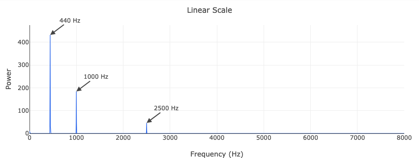
Linear scale

The linear PSD plot shows power concentrated at the three input frequencies. Because PSD squares the amplitude, the ratio between peaks is exaggerated compared to the magnitude spectrum: the 440 Hz tone (amplitude 1.0, power 1.0) towers over the 2500 Hz tone (amplitude 0.3, power 0.09).

Power spectral density -- linear scale

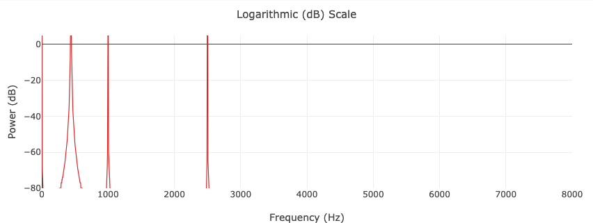
Logarithmic (dB) scale

The dB plot uses \(10 \log_{10}(\text{PSD})\) – note the factor of 10 (not 20) because PSD is already a power quantity. This reveals the noise floor and window side lobes clearly.

Power spectral density -- dB scale

Key takeaways

• PSD measures how power distributes across frequencies; the magnitude spectrum measures amplitude.
• Use \(10 \log_{10}\) for PSD (power) and \(20 \log_{10}\) for magnitude spectrum (amplitude) – both give the same dB values for equivalent signals.
• Parseval's theorem provides a sanity check: the sum of all PSD bins equals the signal's total energy \(\sum x[n]^2\).
• PSD is widely used in noise analysis, SNR estimation, and anywhere you need to quantify the power distribution of a signal.

Further reading

• Spectral density – Wikipedia
• Parseval's theorem – Wikipedia
• Julius O. Smith, Spectral Audio Signal Processing – free online textbook
• Previous tutorial: Computing the Magnitude Spectrum

API reference

• MD_power_spectral_density() – compute the PSD (periodogram)
• MD_magnitude_spectrum() – compute the magnitude spectrum
• MD_Gen_Hann_Win() – generate a Hanning window
• MD_shutdown() – free cached FFTW plans