This tutorial walks through the examples/spectrogram.c program, which generates a linear chirp, computes its STFT with MD_stft(), converts to dB, and writes an interactive HTML heatmap.
If you haven't already, read the Computing the Magnitude Spectrum tutorial first — it covers the DFT fundamentals that the STFT builds on.
What is the STFT?
The magnitude spectrum shows the frequency content of an entire signal. But audio signals are rarely stationary — a speech sentence, a musical phrase, or a chirp sweep all have frequency content that changes over time.
The Short-Time Fourier Transform (STFT) solves this by dividing the signal into short, overlapping frames and computing the DFT of each one. The result is a two-dimensional time-frequency representation called a spectrogram.
For frame \(f\) and frequency bin \(k\), the STFT is:
\[X_f(k) = \sum_{n=0}^{N-1} w[n]\, x[f \cdot H + n]\, e^{-j 2\pi k n / N} \]
Reading the formula in C:
where:
- \(N\) is the FFT window size (samples per frame)
- \(H\) is the hop size (samples between successive frames)
- \(w[n]\) is the Hanning window
- \(x[\cdot]\) is the input signal
MD_stft() stores \(|X_f(k)|\) in a row-major matrix: mag_out[f * (N/2+1) + k].
Time-frequency resolution trade-off
Choosing \(N\) involves a fundamental trade-off:
| Narrow window (small N) | Wide window (large N) | |
|---|---|---|
| Time resolution | High | Low |
| Frequency resolution | Low | High |
| Bins | Few | Many |
A common starting point for speech and music at 16 kHz is \(N = 512\) (32 ms), which gives adequate resolution in both dimensions.
The hop size \(H\) controls frame overlap. 75% overlap ( \(H = N/4\)) is a standard choice that produces smooth spectrograms without excessive computation.
Step 1: Generate a chirp signal
A linear chirp sweeps instantaneous frequency from \(f_0\) to \(f_1\) linearly over a duration \(T\):
\[x(t) = \sin\!\left(2\pi \left(f_0 + \frac{f_1 - f_0}{2T}\,t\right) t\right) \]
Reading the formula in C:
A chirp is the ideal test signal for a spectrogram because its instantaneous frequency changes over time, producing a clearly visible diagonal stripe across the time-frequency plane.
Step 2: Compute the STFT
MD_stft_num_frames() tells you how many complete frames fit in the signal, so you can allocate the output buffer before calling MD_stft().
MD_stft() applies the Hanning window internally, so the signal does not need to be pre-windowed. The output mag_out is a row-major matrix with num_frames rows and N/2+1 columns. Magnitudes are raw FFTW output — not normalised by \(N\).
Step 3: Convert to dB
Raw magnitudes span many orders of magnitude. A log scale compresses the dynamic range and makes both loud and quiet features visible simultaneously.
Normalise by \(N\) before taking the log so that a full-scale sine (amplitude 1) reads near 0 dB. Floor at \(10^{-6}\) to avoid \(\log(0)\).
The formula 20 log \(_{10}\) is used because the input is a magnitude (amplitude), not a power.
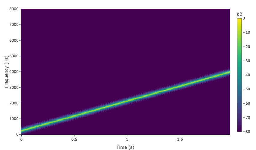
Results
The resulting spectrogram shows the chirp as a diagonal stripe rising from 200 Hz at \(t = 0\) to 4000 Hz at \(t = 2\) s. Hover over the interactive plot to read exact time, frequency, and dB values.
Key takeaways
- The STFT slides a windowed FFT over a signal to reveal how its frequency content evolves over time.
- Window size \(N\) controls the time-frequency trade-off: larger \(N\) gives finer frequency resolution but coarser time resolution.
- Hop size \(H < N\) creates overlapping frames. 75% overlap ( \(H = N/4\)) is a common default.
- MD_stft() reuses the same cached FFT plan as MD_magnitude_spectrum() and MD_power_spectral_density(), so mixing calls with the same \(N\) incurs no extra plan-rebuild overhead.
- Divide magnitudes by \(N\) before dB conversion so that a unit-amplitude sine reads near 0 dB.
Further reading
- Short-time Fourier transform — Wikipedia
- Spectrogram — Wikipedia
- Julius O. Smith, Spectral Audio Signal Processing — free online textbook
- Previous tutorial: Computing the Power Spectral Density
API reference
- MD_chirp_linear() — generate the linear chirp test signal
- MD_stft() — compute the STFT magnitude matrix
- MD_stft_num_frames() — compute the number of output frames
- MD_magnitude_spectrum() — single-frame magnitude spectrum
- MD_power_spectral_density() — single-frame PSD
- MD_Gen_Hann_Win() — generate a Hanning window
- MD_shutdown() — free cached FFTW plans