STFT & Spectrogram
The magnitude spectrum reveals frequency content across an entire signal, but cannot show how that content changes over time. The Short-Time Fourier Transform (STFT) solves this by dividing the signal into short, overlapping frames and computing the DFT of each one, producing a 2-D time-frequency representation called a spectrogram.
Key parameters
Window size (n) — larger windows give better frequency resolution
but worse time resolution. For audio at 16 kHz, n=512 (32 ms) is
a balanced starting point.
Hop size (hop) — controls frame overlap. 75% overlap
(hop = n // 4) is the standard choice: smooth spectrograms without
excessive computation.
Example
import pyminidsp as md
import numpy as np

sr = 16000.0
N = 16000  # 1 second

# Linear chirp — frequency rises from 200 Hz to 4 kHz
signal = md.chirp_linear(N, amplitude=1.0, f_start=200.0,
                          f_end=4000.0, sample_rate=sr)

n = 512
hop = 128
spec = md.stft(signal, n=n, hop=hop)

# spec.shape == (num_frames, n // 2 + 1)
num_frames = md.stft_num_frames(N, n, hop)

# Convert bin k to Hz:  freq_hz = k * sr / n
# Convert frame f to seconds:  time_s = f * hop / sr
Converting to dB
Normalise by n before taking the log so that a full-scale sine (amplitude 1) reads near 0 dB:
spec_db = 20 * np.log10(spec / n + 1e-12)
Visualisation
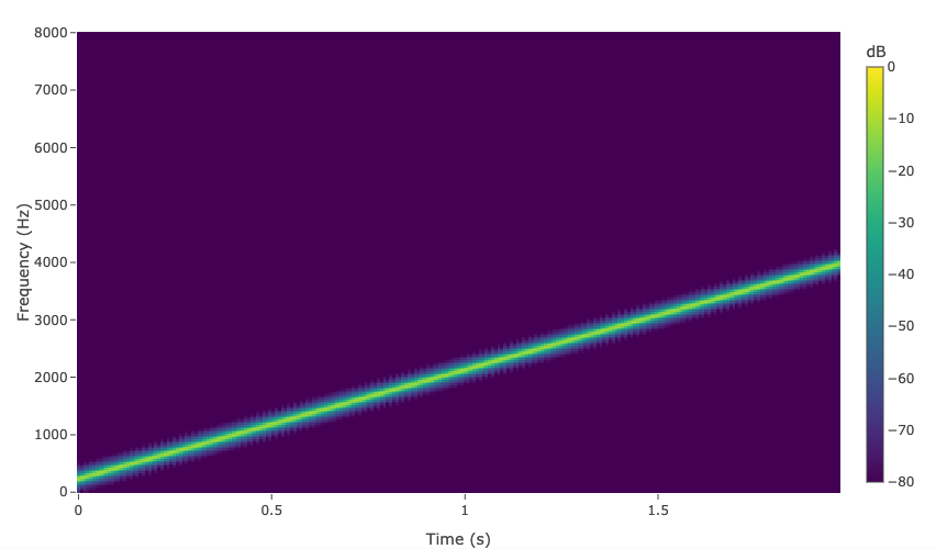
The linear chirp appears as a diagonal stripe rising across the time-frequency plane.
md.shutdown()